1. Adversarial Examples Are Not Bugs, They Are Features
Source: https://arxiv.org/abs/1905.02175
Authors: Andrew Ilyas, Shibani Santurkar, Dimitris Tsipras, Logan Engstrom, Brandon Tran, Aleksander Madry
Topics: deep learning, adversarial examples
Adversarial examples – inputs that are slightly perturbed by an imperceptible noise but causing weird behaviour in machine learning models – have received a great attention, especially since its appearance in the context of deep learning (Szegedy et al. 2013, Goodfellow et al. 2014).
The impact of such examples has also been studied in some previous work (Dalvi et al. 2003,Globerson and Roweis 2006).
The figure below shows one example of adversarial examples including its unintended behaviour.
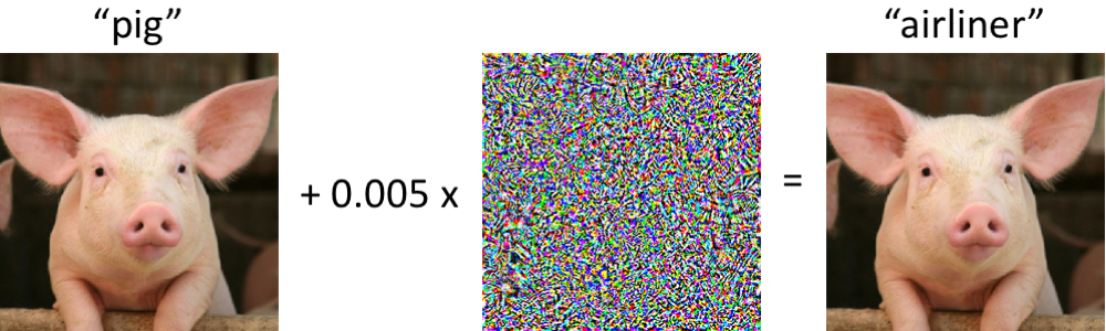
The effect of adversarial noise
To alleviate such a behaviour, some solutions have been proposed, which mainly focus on building more robust models against the adversarial examples (Madry et al. 2018, Stutz et al. 2019)– the solutions theirselves now have a name called adversarial training.
The assumption held by those work is that adversarial examples will disappear if better algorithms and larger scale data are available.
This paper provides a new perspective on why adversarial examples arise in the first place.
The main observation in this work is the existence of the so-called “non-robust features”, which directly attribute to adversarial examples.
Non-robust features are defined as those that are highly predictive, yet brittle and incomprehensible to humans, as opposed to robust features, i.e., highly predictive and also human comprehensible.
This work captures the non-robust features within a theoretical framework and also finds their empirical evidence on a range of image datasets.
The way to find was conducted by disentangling robust and non-robust features via an optimization that results in two separate datasets: robust dataset \(\mathcal{\hat{D}}_R\) and non-robust dataset \(\mathcal{\hat{D}}_{NR}\).
One interesting outcome from this work is that a classifer trained on the robust dataset \(\mathcal{\hat{D}}_R\) through standard training can already reach a certain level of robustness, i.e., having a good adversarial performance.
Additionally, non-robust datasets are found to be sufficient to produce good standard generalisation tests, but suffer from adversarial tests.
The following figure succinctly summarizes the fore-mentioned outcomes.
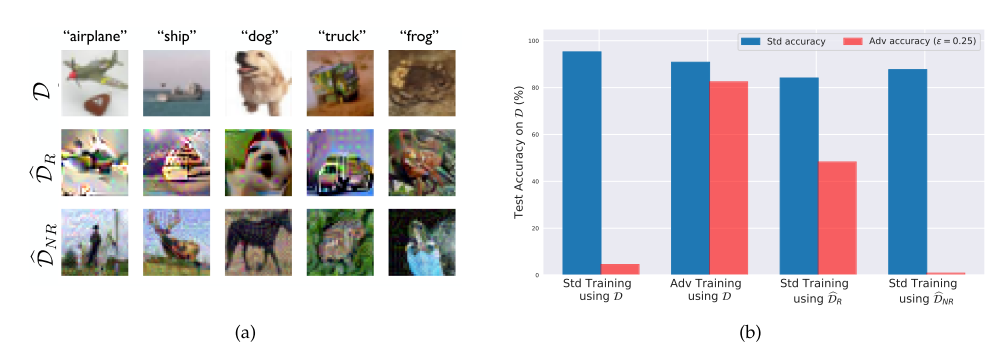
Robust vs non-robust features with respect to the standard and adversarial training
2. Billion-scale Commodity Embedding for E-commerce Recommendation in Alibaba
Source: https://arxiv.org/pdf/1803.02349.pdf
Authors: Jizhe Wang, Pipei Huang, Zhibo Zhang, Binqiang Zhao, Huan Zhao, Dik Lun Lee
Topics: recommender system, graph embedding
Recommender System (RS) is perhaps one of the most widely used AI applications on the Internet these days.
It plays a central role in many business products, especially e-commerces.
This paper proposes an RS solution for Taobao, the largest customer-to-customer (C2C) platform in China to date, that attempts to address three challenges: scalability, sparsity, and cold-start.
In general, the overall system has two stages: 1) matching and 2) ranking.
This paper focuses on addressing the challenges in the matching stage, where the core task is the computation of pairwise similarities between all items based on users’ behaviors.
Such a computation utilizes an embedding derived from graph, namely Base Graph Embedding (BGE), that serves a similar goal as the standard collaborative filtering (CF) based methods but offers higher-order similarities between items.
The graph \(\mathcal{G} = (\mathcal{V}, \mathcal{E})\) is constructed from the behavior history of one billion users within a session or time window, which is one of the main contributions of this paper.
The nodes of the graph represent the items, where each edge is weighted by the co-occurences of the two connected items in all users’ behaviors.
The constructed graph is then used to generate the samples of item sequences based on random walk.
The actual embedding is created through the Skip-gram model (Mikolov et al. 2013) learned from the samples from random walk.
The latter steps are adopted from DeepWalk (Perozzi et al. 2014).
The figure below illustrates the Base Graph Embedding process.
Furthermore, the BGE is also enhanced by incorporating side information, e.g., category, shop, price, etc, of an item, to reduce the cold-start problem.
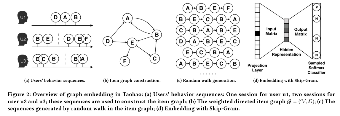
Base Graph Embedding
The overall system was evaluated both in offline (on the link prediction task) and online (under A/B testing framework) fashions.
The experiments show the superiority of the BGE based RS over the existing systems.
3. Greedy InfoMax for Biologically Plausible Self-Supervised Representation Learning
Source: https://arxiv.org/pdf/1905.11786.pdf
Authors: Sindy Lowe, Peter O’Connor, Bastiaan S. Veeling
Topics: deep learning, self-supervision, greedy layerwised training
Modern deep learning models typically rely on the end-to-end supervised training via back-propagation.
There are at least two concerns arising with that approach.
Firstly, it is considered to be not quite biologically plausible.
Secondly, which is more important for practical purposes, it normally needs a large amount of labeled data to train a powerful model.
We all know that labeled data can be expensive to obtain.
This paper proposes a novel algorithm to train a deep neural network in a local, self-supervised mode, referred to as Greedy InfoMax (GIM).
That is, the model is trained in a greedy, modular fashion, i.e., training one module at a time through a self-supervision loss namely InfoNCE loss, adopted from Contrastive Predictive Coding (CPC) (Oord et al. 2018).
Such a modular training is considered to be more biologically plausible (Linsker 1988, [http://www.romanpoet.org/223/Linsker.SelfOrg.pdf], Palmer et al. 2015).
Furthermore, the self-supervision means that the model does not require labeled training data to construct useful representations.
The experiment results show that GIM provides even better accuracy than the fully supervised back-propagation on the STL-10 object classification task.
The accuracy is virtually similar to CPC, except that GIM trains the network module by module, which offers a practical benefit, i.e.,.
decreasing the memory costs during training.
The similar trend of outcomes also can be obseved on the audio classification tasks.
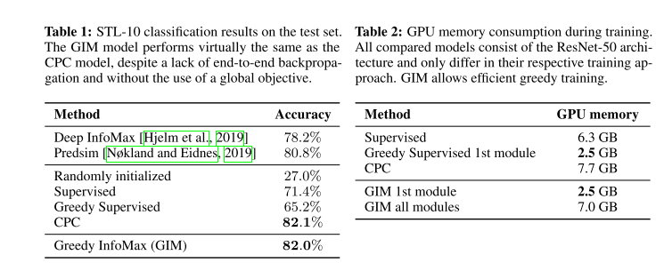
GIM evaluation on STL-10 dataset