flowchart LR
    classDef recurrent fill:#f1f5f9,stroke:#64748b,stroke-width:1.5px,color:#0f172a;
    classDef transformer fill:#f5f3ff,stroke:#8b5cf6,stroke-width:1.5px,color:#4c1d95;
    classDef hybrid fill:#ecfeff,stroke:#0891b2,stroke-width:1.5px,color:#164e63;
    classDef winner fill:#ecfdf5,stroke:#059669,stroke-width:2.5px,color:#064e3b;
    classDef vlm fill:#fff1f2,stroke:#e11d48,stroke-width:1.5px,stroke-dasharray:4 4,color:#881337;

    A["<b>Recurrent Baseline (2016)</b><br/>CRNN: CNN + BiLSTM + CTC"]:::recurrent --> B["<b>Autoregressive ViTs (2021)</b><br/>TrOCR: ViT + Transformer Decoder<br/><i>(High accuracy, slow inference)</i>"]:::transformer
    B --> C["<b>Visual Sequence Hybrids (2022-2025)</b><br/>SVTR & SVTRv2: Visual Mixing + CTC<br/><i>(Fast, non-recurrent, linear decode)</i>"]:::hybrid
    C --> D["<b>Lightweight System Co-Design (2026)</b><br/>PP-OCRv6: PPLCNetV4 + LightSVTR + CTC<br/><i>(1.5M - 34.5M parameters)</i>"]:::winner
    D <--> E["<b>The VLM Counter-Trend (2024-2026)</b><br/>0.9B - 70B Vision-Language Models<br/><i>(Heavy VRAM, ~2,000ms latency, hallucination risk)</i>"]:::vlm
Building Efficient OCR for Clinical Handwriting with JAX
machine-learning
computer-vision
deep-learning
implementation
jax
research-notes
A deep dive into porting PP-OCRv6 to JAX/Flax NNX, verifying numerical parity, and fine-tuning a lightweight CTC recognizer on RxHandBD prescription crops to outperform 0.9B Vision-Language Models on edge CPUs.
Physician handwriting is notoriously difficult to decipher. Cursive flourishes, non-standard clinical abbreviations, and rapid pen strokes challenge even experienced pharmacists. In healthcare, however, transcription mistakes carry real risks: confusing milligrams (mg) with micrograms (mcg) is a thousandfold dosing error, and misreading look-alike drug names such as Celebrex (an anti-inflammatory) for Celexa (an antidepressant) can endanger patients.
Recent Vision-Language Models (VLMs) can read text zero-shot with remarkable fluency, but they bring practical trade-offs. Scaling from 0.9B to 70B parameters, they require heavy GPU compute, introduce multi-second latencies per image, and occasionally hallucinate plausible-sounding drug names when visual evidence is faint. In point-of-care clinics and community pharmacies, where compute is limited to commodity CPUs and patient privacy rules discourage sending scans to external cloud APIs, we need another approach: compact, specialized models that run locally in milliseconds with verifiable visual grounding.
In this post, we explore how to build and adapt an efficient handwriting recognizer using JAX and Flax NNX. We port the lightweight PP-OCRv6 medium recognition model (~34.5M parameters) from Paddle to JAX, verify numerical parity down to floating-point tolerances, and fine-tune it on RxHandBD—a benchmark of 5,578 handwritten prescription crops from doctors in Bangladesh.
By adapting the model using Connectionist Temporal Classification (CTC), we reduce held-out Character Error Rate (CER) from 34.48% to 26.20% and boost Normalized Exact Match from 32.65% to 44.93%. Crucially, this compact recognizer processes word crops in ~52 ms on a standard CPU, outperforming 0.9B parameter VLMs (such as GLM-OCR at 32.8% CER and PaddleOCR-VL-0.9B at 42.44% CER) at a fraction of the computational footprint.
TipOpen-Source Code Repository
All implementation code, configuration files, checkpoint conversion routines, and evaluation manifests for this experiment are publicly available in the ocrax repository: - 🐙 GitHub: github.com/ghif/ocrax - ⚡ Core Stack: JAX, Flax NNX, Optax, Orbax Checkpoint, NumPy, Pillow - 📦 Model & Data: Converted PP-OCRv6 medium recognizer and RxHandBD clinical handwriting manifests
WarningScope and Clinical Safeguards
This project evaluates pre-cropped handwritten word images from medical prescriptions. It focuses specifically on the visual sequence recognition stage; it does not perform full-page document layout analysis, text detection, line segmentation, or medication reconciliation.
While fine-tuning yields substantial accuracy gains, a 60.31% Word Error Rate (WER) remains on isolated words. In safety-critical clinical settings, standalone OCR predictions must always be treated as a decision-support aid under human pharmacist review, never as an autonomous dispensing mechanism.
OCR Evolution: From Fixed Fonts to Visual Sequences
Machine reading has a rich history spanning over a century. In 1912, Edmund Fournier d’Albe demonstrated the optophone—an experimental reading device that translated scanned typography into audible chords (IEEE Spectrum; Eikvil, 1993). Commercial systems followed in the 1950s, but early algorithms relied on template matching against strictly standardized typefaces like OCR-A and OCR-B.
Gradient-based learning shifted the field toward learning features directly from data. LeNet-5 demonstrated this for constrained postal digits (LeCun et al., 1998). The real leap in unconstrained text recognition came with the Convolutional Recurrent Neural Network (CRNN) (Shi et al., 2016), which paired convolutional feature maps with recurrent sequence modeling (BiLSTM) and Connectionist Temporal Classification (CTC) (Graves et al., 2006). This eliminated the need to segment individual characters before classifying them.
In recent years, the field has split into four distinct architectural paradigms, illustrated in Figure 1:
Figure 1: The architectural evolution of text recognition: from recurrent sequence baselines to autoregressive Transformers, visual sequence hybrids, lightweight co-designed engines, and large Vision-Language Models.
- Recurrent Baselines (CRNN): Combine CNN backbones with BiLSTMs. Effective, but recurrent steps impede parallelization.
- Autoregressive Vision Transformers (TrOCR): Pair a Vision Transformer encoder with an autoregressive language decoder (Li et al., 2021). They achieve strong accuracy but suffer from token-by-token decoding latency and are prone to hallucinations when fine-tuned on small datasets.
- Visual Sequence Models (SVTR / SVTRv2): Replace recurrent networks with patch-based visual self-attention and CTC decoding (Du et al., 2022; Du et al., 2024), achieving non-autoregressive decoding speed.
- Co-Designed Lightweight Recognizers (PP-OCRv6): Combine an ultra-compact convolutional trunk (PPLCNetV4) with a lightweight self-attention neck (LightSVTR) and linear CTC projection (Zhang et al., 2026).
- Multimodal Vision-Language Models (VLMs): Generalist models (e.g., GLM-OCR, PaddleOCR-VL-0.9B) that treat recognition as visual question answering or generative sequence modeling. While flexible, their compute footprint makes edge CPU execution impractical.
For clinical applications on commodity hardware, the lightweight co-design paradigm offers the most practical trade-off between inference speed and accuracy.
Anatomy of the Recognition Task and RxHandBD
Where Isolated Word Recognition Fits
Full document transcription requires an end-to-end multi-stage pipeline, outlined in Figure 2:
flowchart TD
    classDef input fill:#e0f2fe,stroke:#0284c7,stroke-width:1.5px,color:#0369a1;
    classDef det fill:#fef3c7,stroke:#d97706,stroke-width:1.5px,color:#92400e;
    classDef rect fill:#ede9fe,stroke:#6366f1,stroke-width:1.5px,color:#3730a3;
    classDef rec fill:#ecfdf5,stroke:#059669,stroke-width:2.5px,color:#064e3b;
    classDef post fill:#fae8ff,stroke:#a855f7,stroke-width:1.5px,color:#6b21a8;
    classDef out fill:#dcfce7,stroke:#16a34a,stroke-width:2px,color:#14532d;

    A["<b>1. Raw Document Image</b><br/>Scanned prescription sheet"]:::input --> B["<b>2. Text Detection (DBNet++)</b><br/>Differentiable binarization & polygons"]:::det
    B --> C["<b>3. Geometric Rectification</b><br/>Perspective unwarping & orientation correction"]:::rect
    C --> D["<b>4. Text Recognition (Our Focus)</b><br/>Visual feature extraction & CTC sequence modeling"]:::rec
    D --> E["<b>5. Decoding & Lexical Post-Processing</b><br/>Beam search & pharmacopeial ontology matching"]:::post
    E --> F["<b>6. Structured Clinical Record</b><br/>Validated digital medication instruction"]:::out
Figure 2: The decoupled anatomy of end-to-end document OCR, contextualizing the isolated word recognition stage addressed in this work.
- Text Detection: A segmentation network like DBNet++ (Liao et al., 2020) detects text regions as arbitrary oriented bounding polygons.
- Geometric Rectification: Perspective transformations unwarp rotated or curved lines into normalized rectangular crops.
- Text Recognition (Our Focus): The core recognizer maps a rectified word crop into character sequence probabilities.
- Lexical Post-Processing: Decoded text is refined against clinical vocabularies (e.g., RxNorm, SNOMED-CT).
- Structured Record Extraction: Entity extraction maps tokens into clinical fields (medication name, dosage, frequency, duration).
%%{init: {'theme': 'base', 'themeVariables': { 'fontSize': '15px' }}}%%
flowchart LR
    classDef input fill:#e0f2fe,stroke:#0284c7,stroke-width:2px,color:#0369a1;
    classDef prep fill:#fef3c7,stroke:#d97706,stroke-width:2px,color:#92400e;
    classDef backbone fill:#ede9fe,stroke:#6366f1,stroke-width:2.5px,color:#3730a3;
    classDef neck fill:#fae8ff,stroke:#a855f7,stroke-width:2px,color:#6b21a8;
    classDef head fill:#ccfbf1,stroke:#0d9488,stroke-width:2px,color:#115e59;
    classDef decode fill:#ecfccb,stroke:#84cc16,stroke-width:2px,color:#3f6212;
    classDef output fill:#dcfce7,stroke:#16a34a,stroke-width:2.5px,color:#14532d;

    subgraph TIER1["<b>Tier 1: Image Ingestion & Anisotropic Feature Extraction</b>"]
        A["<b>1. RxHandBD Word Crop</b><br/>Scanned clinical handwriting<br/><i>Single word image crop</i>"]:::input
        B["<b>2. Decode & Preprocess</b><br/>BGR order, aspect-ratio resize<br/><i>Tensor: (B, 3, 48, 320)</i>"]:::prep
        C["<b>3. PPLCNetV4 Backbone</b><br/>48× vertical collapse, 8× width stride<br/><i>Feature map: (B, 1, 40, 768)</i>"]:::backbone
        A --> B --> C
    end

    subgraph TIER2["<b>Tier 2: Sequence Modeling, CTC Projection & Decoding</b>"]
        D["<b>4. LightSVTR Sequence Neck</b><br/>1×7 depthwise conv + 2× Self-Attention<br/><i>Sequence: (B, 40, 192)</i>"]:::neck
        E["<b>5. Linear CTC Projection</b><br/>Dense class projection across 18,710 classes<br/><i>Logits: (B, 40, 18710)</i>"]:::head
        F["<b>6. Greedy CTC Decoder</b><br/>Argmax per step & blank collapse<br/><i>Deterministic O(T) decode</i>"]:::decode
        G["<b>7. Recognized Word</b><br/>Target clinical transcription<br/><i>e.g., 'Amoxicillin'</i>"]:::output
        D --> E --> F --> G
    end

    C --> D
Figure 3: Computation flow within the isolated word recognition stage, showing tensor dimensionality at each layer.
In this study, we deliberately isolate the visual recognition stage (Figure 3): given an already cropped word image \(x \in \mathbb{R}^{3 \times H \times W}\), how accurately can the network predict the target text string \(\mathbf{y} = (y_1, \dots, y_U)\)?
Isolating this sub-problem controls for text detection and line segmentation errors, allowing us to evaluate the visual feature representations and sequence decoding mechanics directly.
RxHandBD Benchmark
We conduct our experiments on RxHandBD (Islam, 2024), an open-access clinical handwriting benchmark curated at Bangladesh University of Business and Technology (BUBT):
- Dataset Size: 5,578 cropped word images extracted from real medical prescriptions written by practicing physicians in Bangladesh.
- Vocabulary Diversity: 1,559 unique text entries covering generic pharmaceuticals (e.g., Amoxicillin, Metformin), commercial brand names, clinical instructions, and shorthand notations (
1+0+1,5% dns), with occasional English-Bangla code-switching. - Benchmark Split: An official 80/20 train/test partition:
- Training Partition: 4,463 annotated word images.
- Held-Out Test Partition: 1,115 word images evaluated across all baselines.
For our fine-tuning setup, we subdivide the 4,463 training samples into 3,794 training images (85%) and an internal validation set of 669 images (15%) using seed 20261017. The 1,115 test images remain completely untouched until the final evaluation of our selected checkpoint.
Note
Partitioning Caveat: Because RxHandBD does not include metadata linking crops to individual physician IDs, the benchmark uses a sample-level split rather than a writer-disjoint split. While crops from the same prescription are grouped together where feasible, some stylistic correlations across splits cannot be ruled out. Evaluating on strictly writer-disjoint clinical cohorts remains an important future goal.
How We Measure Performance
We track four complementary string edit metrics across the evaluation corpus:
- Character Error Rate (CER): Total Levenshtein edit distance \(d_{\mathrm{Lev}}\) divided by the total number of ground-truth reference characters: \[\mathrm{CER} = \frac{\sum_{i=1}^N d_{\mathrm{Lev}}(\hat{\mathbf{y}}_i, \mathbf{y}_i)}{\sum_{i=1}^N |\mathbf{y}_i|}\]
- Word Error Rate (WER): Token-level edit distance computed over whitespace-delimited words: \[\mathrm{WER} = \frac{\sum_{i=1}^N d_{\mathrm{Word}}(\hat{\mathbf{y}}_i, \mathbf{y}_i)}{\sum_{i=1}^N |\mathbf{y}_i|_{\mathrm{words}}}\]
- Raw Exact Match: The percentage of predicted strings that match the ground-truth target exactly: \[\mathrm{EM}_{\mathrm{raw}} = \frac{1}{N} \sum_{i=1}^N \mathbb{I}(\hat{\mathbf{y}}_i = \mathbf{y}_i)\]
- Normalized Exact Match: Exact match evaluated after case-folding (converting to lowercase) and collapsing whitespace: \[\mathrm{EM}_{\mathrm{norm}} = \frac{1}{N} \sum_{i=1}^N \mathbb{I}(\operatorname{normalize}(\hat{\mathbf{y}}_i) = \operatorname{normalize}(\mathbf{y}_i))\]
Dissecting the PP-OCRv6 Architecture
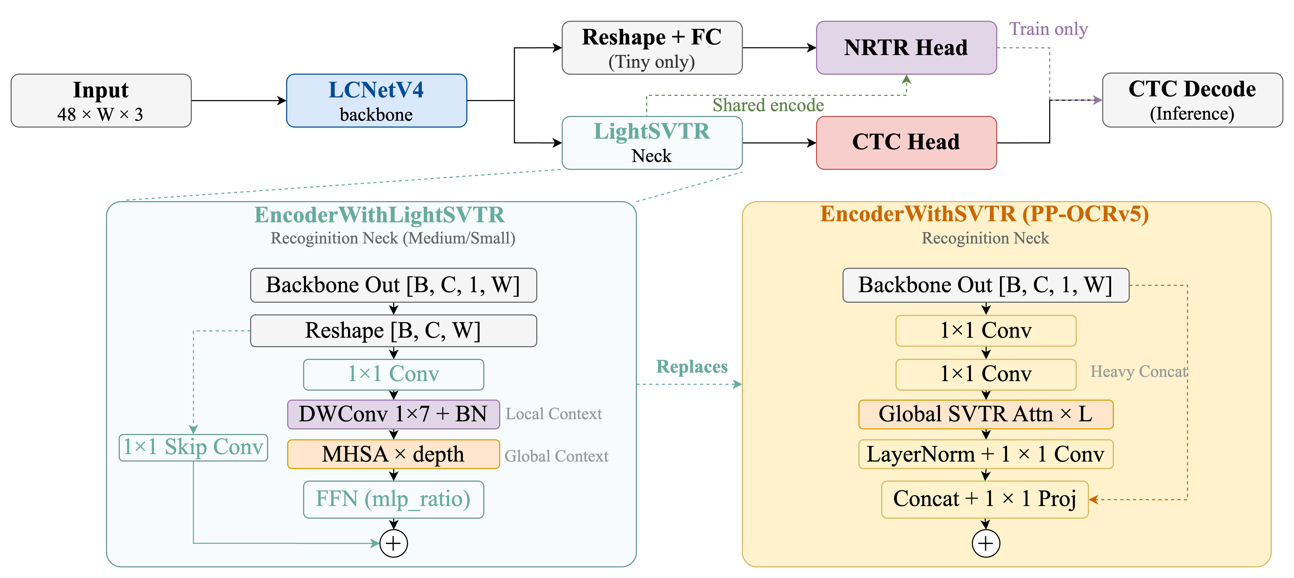
PP-OCRv6 medium recognition couples an ultra-lightweight convolutional trunk with a hybrid self-attention neck and a linear CTC head. Figure 4 displays the complete architecture:
Preprocessing
The recognizer expects a fixed input tensor of shape \(B \times 3 \times 48 \times 320\): 1. Read the input image and convert color channel order to BGR. 2. Resize height to 48 pixels while preserving the original aspect ratio. 3. Clamp width to a maximum of 320 pixels. 4. Right-pad any unused width with zero-intensity pixels. 5. Normalize pixel values to the range \([-1, 1]\).
A critical design choice in PP-OCRv6 is anisotropic downsampling: - Vertical Collapse (\(48\times\)): Height is downsampled aggressively across the backbone stages (\(48 \to 24 \to 12 \to 6 \to 1\)), collapsing 2D visual space into a 1D horizontal feature sequence. - Horizontal Preservation (\(8\times\)): Width is downsampled conservatively (\(320 \to 160 \to 80 \to 40 \to 40\)), preserving \(T = 40\) temporal feature slices.
This asymmetric geometry ensures that receptive fields overlap densely across horizontal pen strokes—providing the spatial resolution needed to distinguish narrow cursive ligatures—while eliminating unnecessary vertical degrees of freedom.
Backbone and Sequence Encoder
The PPLCNetV4 backbone uses depthwise separable convolutions (Howard et al., 2017), Squeeze-and-Excitation (SE) channel recalibration blocks (Hu et al., 2018), and reparameterized depthwise (RepDW) blocks to emit 768 feature channels with minimal multiply-accumulate operations.
A reduction block compresses this feature map from 768 to 192 dimensions. The LightSVTR neck models local horizontal neighborhoods using a \(1 \times 7\) depthwise convolution, followed by two global self-attention blocks (8 heads, MLP expansion ratio of 4, dropout of 0.1) (Du et al., 2022). The resulting sequence of 40 temporal feature vectors is projected via a linear classifier to class logits across \(C = 18{,}710\) classes (18,709 character tokens plus the CTC blank symbol at index 0).
Solving Sayre’s Paradox: Why CTC Matters for Cursive Text
Why did classical OCR algorithms struggle with cursive handwriting? In machine-printed text, whitespace cleanly separates individual letters. Classical systems used vertical projection histograms or connected-component boundaries to slice glyphs into isolated boxes before passing each box to a classifier.
In cursive handwriting, however, adjacent characters are physically connected by continuous ink strokes. This circular dependency was formulated by Richard Sayre in 1973:
“A letter cannot be segmented without being recognized, and cannot be recognized without being segmented.” — Sayre’s Paradox (Sayre, 1973)
An ambiguous stroke (such as cl versus d, or u versus v) cannot be segmented into separate bounding boxes without knowing the linguistic identity of the word; conversely, the identity of the word cannot be recognized without identifying its letters. Slicing cursive text heuristically leads to fragmented or merged characters.
Modern deep OCR resolves Sayre’s Paradox by abandoning character segmentation entirely. Instead of cutting the image into glyphs, the network treats the horizontal spatial dimension as a continuous sequence of time slices, aligning unsegmented frames directly with target text strings using Connectionist Temporal Classification (CTC) (Graves et al., 2006).
%%{init: {'theme': 'base', 'themeVariables': { 'fontSize': '15px' }}}%%
flowchart LR
    classDef logits fill:#f1f5f9,stroke:#64748b,stroke-width:2px,color:#0f172a;
    classDef probs fill:#e0e7ff,stroke:#4f46e5,stroke-width:2px,color:#312e81;
    classDef argmax fill:#fef3c7,stroke:#d97706,stroke-width:2.5px,color:#92400e;
    classDef merge fill:#fae8ff,stroke:#c026d3,stroke-width:2.5px,color:#701a75;
    classDef blank fill:#ffe4e6,stroke:#f43f5e,stroke-width:2.5px,color:#881337;
    classDef clean fill:#dcfce7,stroke:#16a34a,stroke-width:2.5px,color:#14532d;

    subgraph STAGE1["<b>Stage 1: Neural Frame Emission & Greedy Selection</b>"]
        A["<b>1. Frame Logits</b><br/>Unnormalized classifier output<br/><i>Shape: (B, 40, 18710)</i>"]:::logits
        B["<b>2. Softmax Probabilities</b><br/>Framewise class distributions<br/><i>p_t(c|x) at each t ∈ [1, 40]</i>"]:::probs
        C["<b>3. Greedy Frame Argmax</b><br/>Top-1 token ID at each step<br/><i>Example: [ε, h, h, ε, i, i, ε]</i>"]:::argmax
        A --> B --> C
    end

    subgraph STAGE2["<b>Stage 2: Deterministic CTC Sequence Collapse Rule</b>"]
        D["<b>4. Collapse Consecutive Repeats</b><br/>Merge adjacent identical non-blank IDs<br/><i>Example: [ε, h, ε, i, ε]</i>"]:::merge
        E["<b>5. Strip Blank Tokens (ε)</b><br/>Remove all CTC blank delimiters<br/><i>Example: [h, i]</i>"]:::blank
        F["<b>6. Final Transcribed Word</b><br/>Machine-encoded output string<br/><i>Transcribed string: 'hi'</i>"]:::clean
        D --> E --> F
    end

    C --> D
Figure 5: Connectionist Temporal Classification (CTC) sequence decoding and blank-collapse mechanism with running example.
CTC Decoding Mechanics and Blank Collapse
CTC introduces an explicit blank symbol \(\epsilon\) and a collapse operator \(\mathcal{B}\). The collapse rule is straightforward: 1. Merge consecutive identical non-blank tokens. 2. Discard all blank tokens.
For example, an alignment path such as \([\epsilon, h, h, \epsilon, i, i]\) collapses directly to \(hi\).
Under the conditional independence assumption of CTC, the sequence probability is the marginal sum over all valid alignment paths that collapse to target string \(\mathbf{y}\):
\[P(\mathbf{y} \mid x) = \sum_{\boldsymbol{\pi} \in \mathcal{B}^{-1}(\mathbf{y})} \prod_{t=1}^T p_t(\pi_t \mid x)\]
This marginal sum is evaluated efficiently in \(\mathcal{O}(T \cdot U)\) time using the forward-backward dynamic programming algorithm implemented in optax.ctc_loss.
During inference, we convert framewise probabilities into character strings using deterministic greedy decoding (argmax): at each time step \(t \in [1, 40]\), we pick the highest-probability class, merge adjacent identical IDs, and strip blanks. Greedy decoding is computationally lightweight (\(\mathcal{O}(T)\)), requires zero additional memory, and produces deterministic transcriptions.
Re-engineering PP-OCRv6 in JAX and Verifying Parity
PaddleOCR provides a robust production inference runtime, but re-engineering the model in JAX and Flax NNX provides significant advantages for experimentation: 1. Composable Transformations: Native integration with jax.jit for ahead-of-time XLA compilation, jax.grad for reverse-mode differentiation, and jax.vmap for batch vectorization. 2. Modern Flax NNX API: Unlike earlier functional paradigms requiring complex state dictionaries, Flax NNX combines Pythonic object-oriented ergonomics with purely functional execution, making parameters (nnx.Param) and running state (nnx.State) explicit and auditable. 3. Accelerator Portability: Seamless execution across CPUs, Apple Silicon (Metal/MPS), NVIDIA GPUs, and Google Cloud TPUs without modifying model code.
Model Architecture in Flax NNX
In Flax NNX, the complete recognizer is expressed cleanly as an object-oriented module:
import jax
import jax.numpy as jnp
from flax import nnx

class PP_OCRv6MediumRec(nnx.Module):
    """PP-OCRv6 medium recognition inference graph in Flax NNX."""

    def __init__(self, num_classes: int = 18710, rngs: nnx.Rngs | None = None):
        rngs = rngs or nnx.Rngs(0)
        self.backbone = PPLCNetV4Rec("medium", rngs)
        self.neck = LightSVTR(in_channels=768, out_channels=192, depth=2, kernel_size=7, rngs=rngs)
        self.ctc = nnx.Linear(192, num_classes, rngs=rngs)

    def __call__(self, images_nchw: jax.Array, *, training: bool = False) -> jax.Array:
        # Transpose NCHW input to NHWC for standard JAX convolutions
        x = jnp.transpose(images_nchw, (0, 2, 3, 1))
        x = self.backbone(x, training=training)
        x = self.neck(x, training=training)
        # Squeeze spatial height to produce a 1D sequence across width: (B, 40, 192)
        sequence = x[:, 0, :, :]
        logits = self.ctc(sequence)
        if training:
            return logits
        return jax.nn.softmax(logits.astype(jnp.float32), axis=-1)
And greedy CTC decoding is implemented to match Paddle’s blank-first index convention:
def ctc_greedy_decode(probabilities: jax.Array, characters: list[str], blank_id: int = 0) -> list[str]:
    """Greedy CTC decode matching PaddleOCR's blank-first character layout."""
    ids = jnp.argmax(probabilities, axis=-1)
    outputs = []
    for row in ids.tolist():
        previous = None
        chars = []
        for token in row:
            if token != previous and token != blank_id:
                chars.append(characters[token - 1])
            previous = token
        outputs.append("".join(chars))
    return outputs
Weight Conversion and Numerical Parity
Weights are only valid if their mathematical relationship to the computational graph is preserved. The conversion pipeline extracts the Paddle Inference Representation (PIR) parameter graph, exports parameters to an NPZ archive, and maps them into Flax NNX state (Figure 6):
flowchart TD
    classDef paddle fill:#e0f2fe,stroke:#0284c7,stroke-width:1.5px,color:#0369a1;
    classDef seam fill:#fef3c7,stroke:#d97706,stroke-width:1.5px,color:#92400e;
    classDef jax fill:#ede9fe,stroke:#6366f1,stroke-width:1.5px,color:#3730a3;
    classDef parity fill:#dcfce7,stroke:#16a34a,stroke-width:2px,color:#14532d;

    subgraph PADDLE["<b>Paddle Inference Domain</b>"]
        A["Paddle PIR program and parameters"]:::paddle
        B["Export named arrays"]:::paddle
    end

    subgraph SEAM["<b>Conversion & Transformation Seam</b>"]
        C["Map names and transpose layouts"]:::seam
    end

    subgraph JAX["<b>JAX / Flax NNX Runtime Domain</b>"]
        D["Assign Flax NNX state"]:::jax
        E["Save Orbax checkpoint"]:::jax
    end

    subgraph PARITY["<b>Numerical Parity Harness</b>"]
        F["Run same tensors through Paddle and JAX"]:::parity
        G["Compare logits, probabilities, and argmax IDs"]:::parity
    end

    A --> B
    B --> C
    C --> D
    D --> E
    E --> F
    F --> G
Figure 6: The Paddle-to-JAX weight conversion, layout transposition, and numerical parity verification pipeline.
Kernel Layout Permutation: Paddle stores 2D convolution kernels in
O × I × H × Wlayout, whereas Flax convolutions expectH × W × I × O. We permute axes via transpose:def paddle_oihw_to_flax_hwio(weight): """Convert a Paddle Conv2D kernel to Flax HWIO layout.""" return weight.transpose(2, 3, 1, 0)Fused Normalization Layers: In the exported PIR inference graph, batch normalization running statistics are already folded into convolution weights and biases. We preserve these affine transformations while freezing running statistics.
Parity Verification: All 161 of 161 parameter tensors were accounted for and saved as an Orbax checkpoint. We evaluated parity across nine test inputs under strict tolerances (
atol = 2e-4,rtol = 2e-4). Across all \(9 \times 40 = 360\) temporal steps over 18,710 classes, JAX predictions achieved 360 of 360 matching argmax IDs, with a maximum absolute probability deviation of only \(\epsilon_{\max} \approx 3.348 \times 10^{-4}\).
Fine-Tuning Recipe: Adapting CTC to Handwriting
Adapting the converted recognizer to RxHandBD optimizes the CTC loss directly on the deployed inference graph. In this section, we break down the mathematics of the CTC alignment algorithm, how the forward-backward dynamic program computes exact gradients, and how the optimization loop is implemented in JAX and Flax NNX.
Alignment Challenges in Clinical Cursive
In standard sequence classification (such as machine translation or image captioning), target tokens correspond to discrete steps in an autoregressive decoder. In unsegmented text recognition, however, we face an alignment challenge: for an input image \(x\) transformed into \(T = 40\) horizontal feature slices and a target word \(\mathbf{y} = (y_1, y_2, \dots, y_U)\), we do not have character-level bounding boxes or ground-truth alignments indicating which of the 40 time steps corresponds to each letter.
For an alphabet \(\Sigma\), let \(\Sigma' = \Sigma \cup \{\epsilon\}\) denote the character set augmented with the CTC blank token \(\epsilon\). At each frame \(t \in [1, T]\), the model outputs unnormalized logits \(z_t \in \mathbb{R}^{C}\) (where \(C = |\Sigma'| = 18{,}710\)), normalized via softmax into conditional token probabilities:
\[p_t(c \mid x) = \frac{\exp(z_{t,c})}{\sum_{k=0}^{C-1}\exp(z_{t,k})}\]
An alignment path \(\boldsymbol{\pi} = (\pi_1, \pi_2, \dots, \pi_T) \in (\Sigma')^T\) represents an assignment of tokens across all 40 time steps. Under CTC’s conditional independence assumption across frames, the probability of path \(\boldsymbol{\pi}\) is:
\[P(\boldsymbol{\pi} \mid x) = \prod_{t=1}^T p_t(\pi_t \mid x)\]
The collapse operator \(\mathcal{B}: (\Sigma')^T \to \Sigma^{\le T}\) maps an alignment path \(\boldsymbol{\pi}\) to a discrete transcription by merging consecutive identical non-blank characters and then discarding all blanks (e.g., \(\mathcal{B}(\epsilon, a, a, \epsilon, b, b) = ab\)). The probability of the target word \(\mathbf{y}\) is the marginal sum over all valid paths that collapse to it:
\[P(\mathbf{y} \mid x) = \sum_{\boldsymbol{\pi} \in \mathcal{B}^{-1}(\mathbf{y})} P(\boldsymbol{\pi} \mid x)\]
The objective is to minimize the negative log-likelihood of the ground-truth sequence:
\[\mathcal{L}_{\mathrm{CTC}} = -\log P(\mathbf{y} \mid x)\]
Forward-Backward Dynamic Programming
Directly evaluating the marginal sum \(\sum_{\boldsymbol{\pi} \in \mathcal{B}^{-1}(\mathbf{y})}\) is computationally intractable: for \(|\Sigma'| = 18{,}710\) and \(T = 40\), there are \(18{,}710^{40}\) candidate paths. CTC overcomes this using a dynamic programming algorithm that evaluates the marginal likelihood in \(\mathcal{O}(T \cdot U)\) time.
Expanded Label Sequences with Interleaved Blanks
To distinguish between repeated letters (e.g., the double l in penicillin) and letters held across multiple frames, CTC constructs a modified target sequence \(\mathbf{l}'\) by interleaving blank tokens \(\epsilon\) at the beginning, end, and between every character of \(\mathbf{y}\):
\[\mathbf{l}' = (\epsilon, y_1, \epsilon, y_2, \epsilon, \dots, \epsilon, y_U, \epsilon)\]
The expanded sequence has length \(U' = 2U + 1\). For example, the four-letter drug prefix amox (\(U = 4\)) expands into a 9-token sequence:
\[\mathbf{l}' = (\epsilon, a, \epsilon, m, \epsilon, o, \epsilon, x, \epsilon)\]
Forward Variable \(\alpha_t(s)\)
We define the forward variable \(\alpha_t(s)\) as the total probability of all length-\(t\) prefix paths that collapse to the sub-sequence \(\mathbf{l}'_{1:s}\):
\[\alpha_t(s) = \sum_{\substack{\boldsymbol{\pi}_{1:t} \\ \mathcal{B}(\boldsymbol{\pi}_{1:t}) = \mathbf{l}'_{1:s}}} \prod_{\tau=1}^t p_\tau(\pi_\tau \mid x)\]
Base Cases (\(t = 1\))
Any valid alignment must start either with the initial blank \(\mathbf{l}'_1 = \epsilon\) or the first character \(\mathbf{l}'_2 = y_1\). All other states are unreachable at the first frame:
\[\alpha_1(1) = p_1(\epsilon \mid x), \qquad \alpha_1(2) = p_1(y_1 \mid x), \qquad \alpha_1(s) = 0 \quad \forall s > 2\]
Recursive State Transitions (\(t > 1\))
At time step \(t\), the state \(s\) on the expanded sequence \(\mathbf{l}'\) can be reached through three possible transitions: 1. Self-loop: Remaining on the same label \(\mathbf{l}'_s\) from state \(s\) at time \(t-1\). 2. Sequential step: Transitioning from the previous label \(\mathbf{l}'_{s-1}\) at time \(t-1\). 3. Blank skip: Jumping over an intermediate blank from state \(s-2\) at time \(t-1\).
Crucially, skipping a blank is only permissible if \(\mathbf{l}'_s\) is not a blank and differs from the character two steps prior (\(\mathbf{l}'_s \ne \mathbf{l}'_{s-2}\)). If \(\mathbf{l}'_s = \mathbf{l}'_{s-2}\) (e.g., moving between the two consecutive l characters in cloxacillin), the intervening blank \(\epsilon\) is structurally mandatory—skipping it would cause the two consecutive identical characters to merge into a single character under \(\mathcal{B}\).
This yields the complete forward recurrence:
\[\alpha_t(s) = \begin{cases} \left[ \alpha_{t-1}(s) + \alpha_{t-1}(s-1) \right] p_t(\mathbf{l}'_s \mid x), & \text{if } \mathbf{l}'_s = \epsilon \text{ or } \mathbf{l}'_s = \mathbf{l}'_{s-2} \\ \left[ \alpha_{t-1}(s) + \alpha_{t-1}(s-1) + \alpha_{t-1}(s-2) \right] p_t(\mathbf{l}'_s \mid x), & \text{otherwise} \end{cases}\]
Total Sequence Likelihood
Because a complete transcription can validly end either on the final character \(\mathbf{l}'_{2U} = y_U\) or on the trailing blank \(\mathbf{l}'_{2U+1} = \epsilon\), the total sequence probability is simply the sum of the final two states at time \(T\):
\[P(\mathbf{y} \mid x) = \alpha_T(2U) + \alpha_T(2U+1)\]
Backward Variable \(\beta_t(s)\)
Symmetrically, the backward variable \(\beta_t(s)\) computes the probability of all suffix paths from time \(t\) to \(T\) that complete the transcription given that state \(s\) was reached at time \(t\):
\[\beta_T(2U) = 1, \qquad \beta_T(2U+1) = 1, \qquad \beta_T(s) = 0 \quad \forall s < 2U\]
\[\beta_t(s) = \begin{cases} \left[ \beta_{t+1}(s) p_{t+1}(\mathbf{l}'_s \mid x) + \beta_{t+1}(s+1) p_{t+1}(\mathbf{l}'_{s+1} \mid x) \right], & \text{if } \mathbf{l}'_s = \epsilon \text{ or } \mathbf{l}'_s = \mathbf{l}'_{s+2} \\ \left[ \beta_{t+1}(s) p_{t+1}(\mathbf{l}'_s \mid x) + \beta_{t+1}(s+1) p_{t+1}(\mathbf{l}'_{s+1} \mid x) + \beta_{t+1}(s+2) p_{t+1}(\mathbf{l}'_{s+2} \mid x) \right], & \text{otherwise} \end{cases}\]
By tabulating \(\alpha_t(s)\) and \(\beta_t(s)\) across a \(T \times (2U+1)\) lattice, CTC evaluates sequence likelihood in \(\mathcal{O}(T \cdot U)\) steps. For an average handwritten word (\(U \approx 6, T = 40\)), the lattice requires only \(40 \times 13 = 520\) cell evaluations.
Analytic Logit Gradient: Prediction Minus Posterior
To update model parameters \(\theta\) via backpropagation, we differentiate \(\mathcal{L}_{\mathrm{CTC}} = -\log P(\mathbf{y} \mid x)\) with respect to the unnormalized network logits \(z_{t,c}\).
The product \(\alpha_t(s) \beta_t(s)\) represents the unnormalized probability of all paths that pass through state \(s\) on the expanded sequence \(\mathbf{l}'\) at time step \(t\). Summing over all positions where class \(c\) appears in \(\mathbf{l}'\):
\[\operatorname{pos}(\mathbf{l}', c) = \{s \mid \mathbf{l}'_s = c\}\]
The joint probability that the model emits class \(c\) at time \(t\) along an alignment that successfully collapses to \(\mathbf{y}\) is:
\[P(\pi_t = c, \mathbf{y} \mid x) = \sum_{s \in \operatorname{pos}(\mathbf{l}', c)} \frac{\alpha_t(s) \beta_t(s)}{p_t(c \mid x)}\]
Applying the chain rule through the softmax function, the derivative of \(\mathcal{L}_{\mathrm{CTC}}\) with respect to logit \(z_{t,c}\) simplifies to an elegant closed form:
\[\frac{\partial \mathcal{L}_{\mathrm{CTC}}}{\partial z_{t,c}} = p_t(c \mid x) - \frac{1}{P(\mathbf{y} \mid x)} \sum_{s \in \operatorname{pos}(\mathbf{l}', c)} \alpha_t(s) \beta_t(s)\]
Defining \(\gamma_t(c) = P(\pi_t = c \mid \mathbf{y}, x) = \frac{1}{P(\mathbf{y} \mid x)} \sum_{s \in \operatorname{pos}(\mathbf{l}', c)} \alpha_t(s) \beta_t(s)\) as the posterior alignment probability that class \(c\) accounts for frame \(t\), the gradient becomes:
\[\frac{\partial \mathcal{L}_{\mathrm{CTC}}}{\partial z_{t,c}} = p_t(c \mid x) - \gamma_t(c)\]
This formulation provides an intuitive error signal: - If the model assigns higher probability to class \(c\) than the alignment posterior demands (\(p_t(c \mid x) > \gamma_t(c)\)), the gradient is positive, driving logit \(z_{t,c}\) down. - If the model under-predicts a character that the valid alignment paths require (\(p_t(c \mid x) < \gamma_t(c)\)), the gradient is negative, pushing \(z_{t,c}\) upward.
Batched Loss and Variable-Length Masking in Optax
In a minibatch of size \(B = 8\), word images have variable text lengths \(U_i \le U_{\max}\). To compile efficient execution graphs under JAX, input arrays must maintain static tensor shapes.
optax.ctc_loss handles variable sequence lengths using boolean padding masks: - logits: Tensor of shape \((B, T, C) = (8, 40, 18710)\). - logit_paddings: Binary array of shape \((B, T)\) indicating valid temporal frames (all set to \(0.0\) for active frames). - labels: Integer array of shape \((B, U_{\max})\) padded with trailing zeros (blank class). - label_paddings: Binary array of shape \((B, U_{\max})\) where \(0.0\) denotes a real character and \(1.0\) marks a padding token.
The minibatch objective computes the empirical mean over active samples:
\[L_B(\theta) = \frac{1}{B} \sum_{i=1}^B \mathcal{L}_{\mathrm{CTC}}^{(i)}(\theta)\]
JAX / Flax NNX Training Step Implementation
The complete forward loss computation, functional differentiation, gradient norm clipping, and optimizer step are expressed in JAX as follows:
import jax
import jax.numpy as jnp
from flax import nnx
import optax

@nnx.jit
def train_step(
    model: PP_OCRv6MediumRec,
    optimizer: nnx.Optimizer,
    images: jax.Array,
    labels: jax.Array,
    label_paddings: jax.Array,
) -> tuple[jax.Array, jax.Array]:
    """JIT-compiled CTC training step with global gradient norm clipping."""

    def loss_fn(m: PP_OCRv6MediumRec):
        # Forward pass emits frame logits: shape (B, 40, 18710)
        logits = m(images, training=True)
        logit_paddings = jnp.zeros(logits.shape[:2], dtype=jnp.float32)

        # Evaluate forward-backward CTC loss across the batch
        per_sample_loss = optax.ctc_loss(
            logits=logits,
            logit_paddings=logit_paddings,
            labels=labels,
            label_paddings=label_paddings,
        )
        return jnp.mean(per_sample_loss)

    # Differentiate loss with respect to all trainable model parameters
    loss, grads = nnx.value_and_grad(loss_fn)(model)

    # Global Euclidean norm clipping to prevent gradient divergence on illegible crops
    grad_norm = optax.global_norm(grads)
    clip_factor = jnp.minimum(1.0, 1.0 / (grad_norm + 1e-6))
    clipped_grads = jax.tree.map(lambda g: g * clip_factor, grads)

    # Apply decoupled AdamW update
    optimizer.update(clipped_grads)
    return loss, grad_norm
To stabilize training against gradient spikes caused by illegible or severely distorted handwriting, gradients are clipped by their global Euclidean norm:
\[\tilde{\mathbf{g}} = \mathbf{g} \cdot \min\left(1, \frac{1}{\|\mathbf{g}\|_2}\right)\]
Parameters are updated using AdamW (Kingma and Ba, 2014; Loshchilov and Hutter, 2017) with decoupled weight decay: - Learning rate \(\eta = 5 \times 10^{-6}\) - Weight decay \(\lambda = 10^{-5}\) - Momentum parameters \(\beta_1 = 0.9\), \(\beta_2 = 0.999\), \(\epsilon = 10^{-8}\) - Batch size \(B = 8\)
Parameter State Partitioning: Trainable vs. Frozen Normalization
A central design decision in our fine-tuning recipe is distinguishing between trainable parameters and frozen model statistics:
| Component | State Type | Role in Domain Fine-Tuning |
|---|---|---|
| PPLCNetV4 Trunk | nnx.Param |
Convolution kernels, biases, SE projections, and RepDW weights adapt end-to-end to handwriting stroke features. |
| LightSVTR Neck | nnx.Param |
Channel reduction weights, \(1\times 7\) depthwise filters, self-attention projections, and feed-forward layers adapt to sequence context. |
| CTC Linear Head | nnx.Param |
Dense projection weights (\(192 \to 18{,}710\)) adjust decision boundaries over the character vocabulary. |
| BatchNorm Statistics | nnx.State |
Frozen identity state. Because BatchNorm transformations were folded during conversion, freezing running statistics prevents small minibatches (\(B=8\)) from corrupting learned feature representations. |
Photometric-Only Augmentation
Training images undergo mild photometric perturbations: brightness and contrast scale factors are independently sampled from a uniform distribution \(\mathcal{U}[0.9, 1.1]\).
Importantly, we omit geometric augmentations (affine shearing or warping). In clinical handwriting, pen strokes and diacritical marks are already fragile; synthetic warping risks disconnecting ligatures or blurring fine characters. Validation images use the deterministic, unperturbed transform.
Checkpoint Selection and Early Stopping
Model selection is strictly decoupled from test evaluation (Figure 7):
flowchart TD
    classDef data fill:#e0f2fe,stroke:#0284c7,stroke-width:1.5px,color:#0369a1;
    classDef train fill:#ede9fe,stroke:#6366f1,stroke-width:1.5px,color:#3730a3;
    classDef val fill:#fef3c7,stroke:#d97706,stroke-width:1.5px,color:#92400e;
    classDef decision fill:#fffbeb,stroke:#b45309,stroke-width:2px,color:#78350f;
    classDef save fill:#dcfce7,stroke:#16a34a,stroke-width:2px,color:#14532d;
    classDef warn fill:#ffedd5,stroke:#ea580c,stroke-width:1.5px,color:#7c2d12;
    classDef stop fill:#ffe4e6,stroke:#e11d48,stroke-width:1.5px,color:#881337;
    classDef test fill:#f3e8ff,stroke:#9333ea,stroke-width:2px,color:#581c87;

    A["Train labels only"]:::data --> B["Seeded train and validation manifests"]:::data
    B --> C["Train CTC model on training samples"]:::train
    C --> D["Compute validation CER each epoch"]:::val
    D --> E{"CER improves by min delta?"}:::decision
    E -->|Yes| F["Save selected checkpoint"]:::save
    E -->|No| G["Advance patience counter"]:::warn
    G --> H{"Patience exhausted?"}:::decision
    H -->|No| C
    H -->|Yes| I["Stop training"]:::stop
    F --> J["Evaluate once on held-out test labels"]:::test
Figure 7: Early-stopping and model-selection workflow driven by validation Character Error Rate (CER).
At the end of each epoch, the model evaluates on the 669 unperturbed validation samples to compute corpus CER. A candidate checkpoint is saved only if it improves validation CER by at least \(\delta = 0.001\):
\[\mathrm{CER}_{\text{new}} < \mathrm{CER}_{\text{best}} - 0.001\]
If three consecutive epochs elapse without meeting this threshold (\(\text{patience} = 3\)), training terminates early. In our experiment, the optimal validation CER was achieved at Epoch 14 (16.65% CER, 45.59% Exact Match). Training stopped at epoch 17 (~8.12 hours on CPU), and this epoch-14 checkpoint was frozen for test evaluation.
Benchmark Results: Compact CTC Models vs. 0.9B VLMs
Zero-Shot Baseline Results
Evaluating the converted pretrained PP-OCRv6 checkpoint zero-shot on the 1,115 held-out test crops establishes our baseline:
| Metric | Zero-Shot JAX PP-OCRv6 |
|---|---|
| Raw Exact Match | 28.16% (314 / 1,115) |
| Normalized Exact Match | 32.65% (364 / 1,115) |
| Character Error Rate (CER) | 34.48% |
Word Accuracy (1 - WER) |
28.94% |
| Word Error Rate (WER) | 71.06% |
An earlier pipeline run using PaddleOCR reported 25.92% raw exact match and 36.15% CER. While aggregate figures appear close, individual predictions differed on 702 of the 1,115 images due to distinct image-reading routines (Pillow vs. OpenCV) and color space handling. While our parity tests confirmed identical behavior on identical tensors, subtle differences in image decoding pipelines introduce measurable prediction variance.
CPU Timing Baseline: Processing batches of size 32 took 67.89 seconds (60.89 ms/image, 16.42 images/second), including loading, preprocessing, inference, and greedy decoding.
Fine-Tuned Performance Gains
Evaluating the selected epoch-14 checkpoint on the 1,115 held-out test crops demonstrated substantial improvements across every metric:
| Metric | Pretrained Zero-Shot JAX | Fine-Tuned JAX | Absolute Improvement |
|---|---|---|---|
| Raw Exact Match | 28.16% (314 / 1,115) | 36.59% (408 / 1,115) | +8.43 pp |
| Normalized Exact Match | 32.65% (364 / 1,115) | 44.93% (501 / 1,115) | +12.28 pp |
| Character Error Rate (CER) | 34.48% | 26.20% | -8.28 pp |
Word Accuracy (1 - WER) |
28.94% | 39.69% | +10.75 pp |
Fine-tuned CPU prediction throughput reached 52.59 ms/image (~19.01 images/second at batch size 32). Despite this 8.28 percentage point drop in CER, 60.31% of words still contain at least one error, reiterating that standalone visual recognition cannot provide autonomous clinical transcription without downstream ontology reconciliation.
Comparative Benchmark: How Do Different Paradigms Stack Up?
To understand how our adapted recognizer compares to alternative approaches, we summarize published results and our direct runs on RxHandBD:
| Model / Architecture | Paradigm | Parameter Count | CER (%) ↓ | WER (%) ↓ | Exact Match (Raw / Norm) ↑ | Edge CPU Latency |
|---|---|---|---|---|---|---|
| Tesseract 5 | Legacy LSTM pattern matcher | — | 78.5% | 104.3% | 2.5% / — | ~49 ms |
| EasyOCR | CRNN (CNN + BiLSTM + CTC) | ~10M | 69.5% | 107.4% | 2.6% / — | ~14 ms |
| PaddleOCR-VL-0.9B | Pretrained VLM (Encoder-Decoder) | 0.9B | 42.44% | 81.73% | 23.77% / 27.80% | ~2,012 ms |
| PP-OCRv5 | Pretrained SVTR + CTC | ~5M | 47.7% | 78.9% | 21.4% / — | ~103 ms |
| GLM-OCR | Pretrained VLM (Vision + Decoder) | 0.9B | 32.8% | 80.1% | 32.6% / — | ~141 ms |
| PP-OCRv6 Pretrained | Pretrained JAX (PPLCNetV4 + LightSVTR) | 34.5M | 34.48% | 71.06% | 28.16% / 32.65% | ~60.9 ms |
| Fine-Tuned PP-OCRv6 (Ours) | Adapted JAX (PPLCNetV4 + LightSVTR) | 34.5M | 26.20% | 60.31% | 36.59% / 44.93% | ~52.6 ms |
Note: Figures for Tesseract, EasyOCR, PP-OCRv5, and GLM-OCR are cited from the 2026 comparative prescription benchmark (“How Well Can OCR Read Doctor Handwriting in 2026?”). PaddleOCR-VL-0.9B and PP-OCRv6 figures represent our direct runs on the identical 1,115 test crops.
Four Key Takeaways from the Comparison
- Legacy Engines Fail Completely: Tesseract 5 and EasyOCR produce Word Error Rates above 100% and exact match scores below 3%. Off-the-shelf general OCR cannot segment or decode unconstrained physician cursive.
- Surpassing 0.9B Parameter Vision-Language Models: Prior to targeted domain adaptation, GLM-OCR (0.9B) established the lowest reported zero-shot CER on RxHandBD at 32.8%. Our fine-tuned recognizer reaches 26.20% CER (-6.60 pp) and 36.59% Raw Exact Match (+3.99 pp), while operating with a 26-fold smaller parameter footprint and executing nearly \(3\times\) faster on CPU (~52.6 ms vs. ~141 ms).
- The Autoregressive Overfitting Trap: Several community attempts on Hugging Face have fine-tuned heavy Vision-Encoder-Decoder architectures (like TrOCR checkpoints scaling to ~1.34 GB) on RxHandBD, consistently plateauing between 30% and 35% CER. In clinical handwriting, fine-tuning large autoregressive decoders on small corpora (~4.5k images) causes overfitting and hallucination, where the language model predicts fluent but fictitious drug names over visually faithful stroke evidence.
- Why Our Adaptation Recipe Succeeded:
- Parameter Capacity Alignment: PP-OCRv6 (~34.5M parameters) matches the scale of the 4,463 training samples without parameter explosion.
- Frozen Folded Normalization: Freezing folded BatchNorm state prevents small minibatches (\(B=8\)) from corrupting learned feature distributions.
- Strict Visual Grounding via CTC: Frame-level CTC alignment computes conditional probabilities over spatial slices, grounding predictions in visual ink rather than linguistic hallucination.
- Photometric-Only Perturbation: Preserving stroke geometry protected fine diacritics and ligatures, and early stopping on validation CER captured the true minimum-error checkpoint at epoch 14.
Lessons, Practical Caveats, and What’s Next
Engineering Insights
- Conversion Requires Strict Parity Verification: Serialization alone does not guarantee model equivalence. Verifying tensor accounting (161/161 layers), layout permutations (
OIHWtoHWIO), and numerical parity tolerances (atol,rtol) is essential to prevent silent layer scrambling. - Preprocessing Contracts Directly Affect Accuracy: In handwriting recognition, subtle details (interpolation method, aspect-ratio rounding, padding color) measurably shift predictions. Inference code must mirror training preprocessing exactly.
- Sequence-Length Loss Masking: In the current implementation, all 40 time steps are treated as valid frames in the CTC loss. Explicitly masking right-padded non-informative frames based on original image aspect ratios represents an immediate path for further optimization.
Practical Limitations in Clinical Workflows
- Writer-Disjoint Generalization: Because RxHandBD does not include clinician identifiers, our evaluation was performed on a sample-level split. Evaluating out-of-distribution robustness on writer-disjoint clinical cohorts is required before real-world deployment.
- Multi-Task Pretraining Objective: PP-OCRv6 pretraining incorporates an auxiliary NRTR Transformer decoder head alongside CTC. Investigating whether retaining the auxiliary transformer decoder during initial adaptation accelerates convergence remains an open research question.
- Structured Error Analysis: Future work should quantify confusion frequencies between high-risk medication pairs and critical dosage units (
mgvs.mcg). - End-to-End Pipeline Integration: Translating word recognition into practice requires robust document detection, line segmentation, and human-in-the-loop verification interfaces.
Reproducing the Experiments
The complete pipeline—from data preparation to parameter conversion, numerical parity verification, and CTC fine-tuning—is reproducible using the ocrax CLI:
# 1. Environment setup
conda create -n ocrax python=3.13 && conda activate ocrax
pip install -e ".[paddle]"

# 2. Prepare seeded train and validation manifests
ocrax-prepare-data \
  --dataset-root /path/to/RxHandBD \
  --output-dir data/manifests \
  --validation-fraction 0.15 \
  --seed 20261017

# 3. Export Paddle inference program and convert to Orbax format
ocrax-export-paddle \
  --model-dir /path/to/PP-OCRv6_medium_rec \
  --output /tmp/ppocrv6_params.npz

JAX_PLATFORMS=cpu ocrax-convert \
  --arrays /tmp/ppocrv6_params.npz \
  --output artifacts/checkpoints/ppocrv6_medium_rec_orbax

# 4. Verify numerical parity against Paddle runtime
JAX_PLATFORMS=cpu ocrax-parity \
  --model-dir /path/to/PP-OCRv6_medium_rec \
  --checkpoint artifacts/checkpoints/ppocrv6_medium_rec_orbax \
  --atol 2e-4 --rtol 2e-4 \
  --report outputs/parity-report.json

# 5. Evaluate zero-shot baseline on held-out test crops
JAX_PLATFORMS=cpu ocrax-evaluate-jax \
  --dataset-root /path/to/RxHandBD \
  --model-dir /path/to/PP-OCRv6_medium_rec \
  --checkpoint artifacts/checkpoints/ppocrv6_medium_rec_orbax \
  --batch-size 32 \
  --output outputs/rxhandbd_ppocrv6_jax_predictions.csv

# 6. Fine-tune on RxHandBD with validation CER early stopping
JAX_PLATFORMS=cpu ocrax-train \
  --dataset-root /path/to/RxHandBD \
  --model-dir /path/to/PP-OCRv6_medium_rec \
  --checkpoint artifacts/checkpoints/ppocrv6_medium_rec_orbax \
  --train-manifest data/manifests/train.jsonl \
  --validation-manifest data/manifests/validation.jsonl \
  --output artifacts/checkpoints/ppocrv6_medium_rec_rxhandbd \
  --epochs 20 --batch-size 8 --learning-rate 5e-6 --patience 3 --min-delta 0.001 --seed 20261017

# 7. Evaluate the selected epoch-14 checkpoint on test crops
JAX_PLATFORMS=cpu ocrax-evaluate-jax \
  --dataset-root /path/to/RxHandBD \
  --model-dir /path/to/PP-OCRv6_medium_rec \
  --checkpoint artifacts/checkpoints/ppocrv6_medium_rec_rxhandbd \
  --batch-size 32 \
  --output outputs/rxhandbd_ppocrv6_jax_finetuned_predictions.csv
References & Further Reading
- Zhang, C., et al. (2026). PP-OCRv6: A Practical and Efficient OCR System. arXiv preprint arXiv:2606.13108.
- Islam, M. M. (2024). RxHandBD: A Handwritten Prescription Word Image Dataset. Mendeley Data, V3. DOI: 10.17632/dsb5r6vskg.3.
- Sayre, R. (1973). Machine recognition of handwritten words: A project report. Pattern Recognition, 5(3), 213–228. DOI: 10.1016/0031-3203(73)90044-6.
- Graves, A., Fernández, S., Gomez, F., & Schmidhuber, J. (2006). Connectionist temporal classification: labelling unsegmented sequence data with recurrent neural networks. In Proceedings of the 23rd International Conference on Machine Learning (ICML ’06), 369–376. DOI: 10.1145/1143844.1143891.
- Shi, B., Bai, X., & Yao, C. (2016). An End-to-End Trainable Neural Network for Image-based Sequence Recognition and Its Application to Scene Text Recognition. IEEE Transactions on Pattern Analysis and Machine Intelligence, 39(11), 2298–2304. arXiv:1507.05717.
- Du, Y., Chen, Z., Jia, C., Yin, X., Zheng, T., Li, C., Du, Y., & Jiang, Y. (2022). SVTR: Scene Text Recognition with a Single Visual Model. In Proceedings of the Thirtieth International Joint Conference on Artificial Intelligence (IJCAI-22), 884–890. arXiv:2205.00159.
- Du, Y., Chen, Z., Jia, C., Yin, X., & Jiang, Y. (2024). SVTRv2: CTC Beats Encoder-Decoder Models in Scene Text Recognition. arXiv preprint arXiv:2411.15858.
- Li, M., Lv, T., Chen, J., Cui, L., Lu, Y., Florencio, D., Zhang, C., & Wei, F. (2021). TrOCR: Transformer-based Optical Character Recognition with Pre-trained Models. arXiv preprint arXiv:2109.10282.
- Liao, M., Zou, Z., Wan, Z., Yao, C., & Bai, X. (2020). Real-time Scene Text Detection with Differentiable Binarization and Adaptive Scale Fusion. IEEE Transactions on Pattern Analysis and Machine Intelligence, 44(2), 919–931. arXiv:1911.08947.
- LeCun, Y., Bottou, L., Bengio, Y., & Haffner, P. (1998). Gradient-based learning applied to document recognition. Proceedings of the IEEE, 86(11), 2278–2324. DOI: 10.1109/5.726791.
- Howard, A. G., et al. (2017). MobileNets: Efficient Convolutional Neural Networks for Mobile Vision Applications. arXiv preprint arXiv:1704.04861.
- Hu, J., Shen, L., & Sun, G. (2018). Squeeze-and-Excitation Networks. In Proceedings of the IEEE Conference on Computer Vision and Pattern Recognition (CVPR ’18), 7132–7141. CVPR 2018.
- Kingma, D. P., & Ba, J. (2014). Adam: A Method for Stochastic Optimization. arXiv preprint arXiv:1412.6980.
- Loshchilov, I., & Hutter, F. (2017). Decoupled Weight Decay Regularization. arXiv preprint arXiv:1711.05101.
- Eikvil, L. (1993). Optical Character Recognition. Technical Report, Department of Informatics, University of Oslo. CiteSeerX.
- d’Albe, E. E. F. (1914). On a type-reading optophone. Proceedings of the Royal Society of London, Series A, 90(619), 373–375.
- Smith, R. (2007). An Overview of the Tesseract OCR Engine. In Proceedings of the Ninth International Conference on Document Analysis and Recognition (ICDAR ’07), 629–633. DOI: 10.1109/ICDAR.2007.4376991.
- Kaniel Outis. (2026). How Well Can OCR Read Doctor Handwriting in 2026? DEV Community Comparative Benchmark. DEV.to.
- PaddlePaddle Authors. (2026). PaddleOCR-VL-0.9B Model Card and Documentation. GitHub / Docs.
- Ghifary, M. (2026). OCRax: Efficient Text Recognition in JAX. Open-source software repository. GitHub: ghif/ocrax.